Not so happy looking!
When I got my start working in Haskell (back in the previous millennium), it felt like a kind of miracle that this magic we were writing could be executed at all.
Nowadays, I feel a little cheated if my code doesn’t perform within a small factor of C code.
We get from “it runs!” to “it’s small and fast!” by measuring, tweaking, and measuring again. And again.
And again.
There are two aspects of performance that are of interest to us.
How long does a program or function take?
How much memory does it require?
Let’s start with time.
An old favourite:
module Length where

len0 :: [a] -> Int
len0 (_:xs) = 1 + len0 xs
len0 _      = 0
Yawn, right?
But how long does it take to run?
The standard Haskell tool for timing measurement is a package named criterion.
cabal install criterioncriterion makes it extremely easy to get a benchmark up and running.
import Criterion.Main
import Length

main = defaultMain [ bench "len0" $ whnf len0 [0..100000] ]
If we compile this to an executable, we’ll have a fully usable benchmark program.
The defaultMain function accepts a list of benchmarks to run.
It parses a standard set of command line arguments, then runs the benchmarks.
The bench function describes a single benchmark.
Its first argument is the name to print for the benchmark.
The second is a description of the actual function to benchmark.
The whnf function describes how to run a benchmark.
criterion provides several ways to run a benchmark.
For pure functions:
whnf accepts two arguments, a function and the last argument to pass to the function. It supplies the argument to the function, then evaluates the result to weak head normal form (WHNF).
nf is similar, but evaluates the result to normal form (NF).
For impure IO actions:
whnfIO accepts an IO action, runs it, and evaluates the result to WHNF.
nfIO accepts an IO action, runs it, and evaluates the result to NF.
Ideally, we’d always benchmark on a completely quiet machine with predictable performance.
There are many reasons why this is not achievable, among them:
CPU frequency changes in response to load and thermal stress
Other processes (e.g. web browsers) contending for resources
External interrupts, e.g. from mouse, network adapters
So are we doomed?
While we can’t directly observe sources of measurement interference, we can detect interference that perturbs our measurements.
If the interference is moderate to severe, it will perturb many measurements, and criterion will indicate that its measurements are suspicious.
The output of a criterion run:
benchmarking len0
time                 1.018 ms   (969.8 μs .. 1.062 ms)
                     0.990 R²   (0.987 R² .. 0.995 R²)
mean                 1.022 ms   (999.1 μs .. 1.047 ms)
std dev              76.43 μs   (64.41 μs .. 92.50 μs)
variance introduced by outliers: 60% (severely inflated)criterion works hard to be fully automatic.
It measures the cost of your function multiple times.
Increases the number of calls to your function
Performs linear regression over these measurements
As a result, its accuracy is impressive.
What about these numbers?
benchmarking len0
time                 1.018 ms   (969.8 μs .. 1.062 ms)
                     0.990 R²   (0.987 R² .. 0.995 R²)
mean                 1.022 ms   (999.1 μs .. 1.047 ms)
std dev              76.43 μs   (64.41 μs .. 92.50 μs)
variance introduced by outliers: 60% (severely inflated)
How come we’re giving bounds (969.8 μs .. 1.062 ms) on measurements, and mean and standard deviation?
Measuring is a noisy business. These are estimates of the range within which 95% of our values are falling.
We can get a great start by building our programs with the -rtsopts option. This allows us to pass extra options to GHC’s runtime system when we run our compiled program.
Suppose we want to see the space performance of this program.
import Control.Monad (forM_)
import Data.List (sortBy)
import Data.Ord (comparing)
import System.Environment (getArgs)
import qualified Data.Map as M

main = do
  args <- getArgs
  forM_ args $ \f -> do
    ws <- words `fmap` readFile f
    forM_ (sortBy (comparing snd) . M.toList .
           foldl (\m w -> M.insertWith (+) w 1 m) M.empty $ ws) $
          \(w,c) -> putStrLn $ show c ++ "\t" ++ w
We compile it with the following command line:
ghc -O -rtsopts --make WordFreq.hsThe +RTS command line option begins a series of RTS options. The RTS will hide these from our program.
The -RTS option ends the series of RTS options. (We can omit it if RTS options are the last thing on the command line.)
./WordFreq foo.txt +RTS -s -RTSThe -s RTS option tells the runtime to print summary statistics from the memory manager.
   160,394,496 bytes allocated in the heap
   104,813,280 bytes copied during GC
    15,228,592 bytes maximum residency (9 sample(s))
       328,112 bytes maximum slop
        36 MB total memory in use (0 MB lost due to fragmentation)

                  Tot time (elapsed)  Avg pause  Max pause
Gen  0       297 colls,     0 par    0.10s    0.10s     0.0003s    0.0021s
Gen  1         9 colls,     0 par    0.08s    0.10s     0.0113s    0.0350s

INIT    time    0.00s  (  0.00s elapsed)
MUT     time    0.12s  (  0.13s elapsed)
GC      time    0.18s  (  0.20s elapsed)
EXIT    time    0.00s  (  0.00s elapsed)
Total   time    0.31s  (  0.33s elapsed)

%GC     time      59.1%  (60.7% elapsed)

Alloc rate    1,280,768,615 bytes per MUT second

Productivity 40.9% of total user, 37.6% of total elapsedLet’s break it all down, from top to bottom.
   160,394,496 bytes allocated in the heap
   104,813,280 bytes copied during GC
    15,228,592 bytes maximum residency (9 sample(s))
       328,112 bytes maximum slop
        36 MB total memory in use (0 MB lost due to fragmentation)
Key statistics to look at:
allocated in the heap: total memory allocated during entire run
copied during GC: amount of memory that had to be copied because it was alive
maximum residency: largest amount of memory in use at one time
Time spent in the garbage collector:
                  Tot time (elapsed)  Avg pause  Max pause
Gen  0       297 colls,     0 par    0.10s    0.10s     0.0003s    0.0021s
Gen  1         9 colls,     0 par    0.08s    0.10s     0.0113s    0.0350s
GHC uses a generational GC, so we get a GC breakdown by generation. Gen 0 is the nursery.
par is the number of GC passes that used multiple CPUs in parallel.
Where the program spent its time:
INIT    time    0.00s  (  0.00s elapsed)
MUT     time    0.12s  (  0.13s elapsed)
GC      time    0.18s  (  0.20s elapsed)
EXIT    time    0.00s  (  0.00s elapsed)
Total time 0.31s ( 0.33s elapsed)INIT: starting the program
MUT: “mutation”, the part where the program was doing useful work
GC: garbage collection
EXIT: shutdown
There are two columns of numbers in case we’re running on multiple cores.
These are really the most useful numbers to look at:
%GC     time      59.1%  (60.7% elapsed)

Alloc rate    1,280,768,615 bytes per MUT second

Productivity  40.9% of total user, 37.6% of total elapsed
If GC time is high and productivity is low, we’re spending a lot of time doing GC, which leaves less for real work.
Are the numbers above healthy? NO!
There were problems in our code - but what were they?
Another standard RTS option:
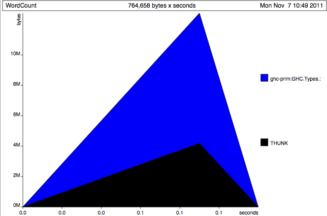
./WordFreq foo.txt +RTS -hTThis generates a file named WordFreq.hp, which contains a heap profile, a time-based snapshot of what was in the heap and when, categorized by data constructor.
We can’t easily read a heap profile, so we use hp2ps to convert it to a PostScript file.
hp2ps -c WordFreq.hpThis will give us WordFreq.ps, which we can open in a suitable viewer.
Not so happy looking!
Clearly we’re allocating a ton of cons cells, and half a ton of thunks.
Does this heap profile look better?
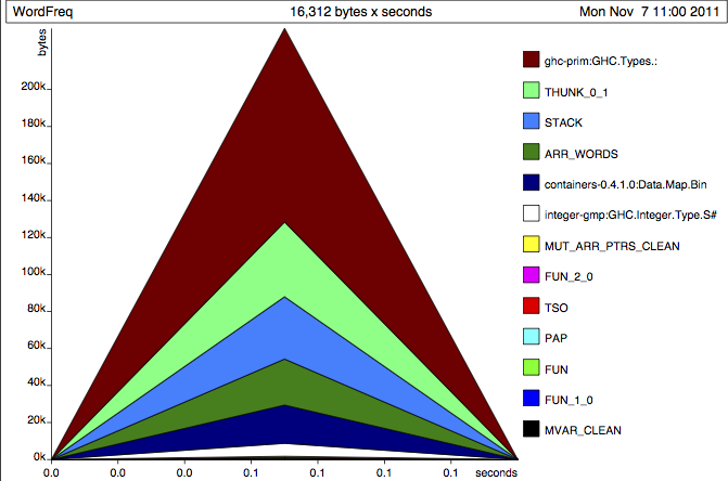
What a relief!
It’s still a similar shape, but look at the units on the y axis above!
Also, check out the healthier GC summary stats:
%GC     time      33.6%  (32.9% elapsed)

Alloc rate    1,246,782,295 bytes per MUT second

Productivity 66.4% of total user, 63.3% of total elapsedBasic heap profiling is useful, but GHC supports a much richer way to profile our code.
This richer profiling support has a space and time cost, so we don’t leave it turned on all the time.
To use it, we must compile both libraries and programs with -prof.
If you’re using cabal, see the --enable-library-profiling and --enable-executable-profiling options.
As mentioned in an early lecture, simply leave library-profiling set to True in your $HOME/.cabal/config.
With library profiling enabled, cabal will generate both normal and profiled libraries, and will use the right one at the right time.
The basics of full heap profiling are similar to what we saw with -hT and hp2ps a moment ago.
The full profiler is a powerful facility, so it’s worth reading the profiling chapter of the GHC manual.
In particular, to get much out of the profiler, you’ll need to know about cost centres, which are annotated expressions used for book-keeping when profiling.
In many cases, you can simply use the -auto-all option to get GHC to annotate all top-level bindings with cost centres.
You’ll also want to use the -P RTS option, which writes a human-readable time and space profile into a file ending with a .prof extension.
criterion lets us look not just at time, but at memory consumption, GC invocations, and a few other interesting things…
Use --help to find out details.
The key is to linearly regress other measurements against number of iterations.
Run code with +RTS -T to enable this.
Given our earlier definition of the function len0, suppose we try this on the command line:
ghc -c -ddump-simpl Length.hsAnd we’ll see GHC dump a transformed version of our code in a language named Core.
Rec {
Length.len0 [Occ=LoopBreaker]
  :: forall a_abp. [a_abp] -> GHC.Types.Int
[GblId, Arity=1]
Length.len0 =
  \ (@ a_aov) (ds_dpn :: [a_aov]) ->
    case ds_dpn of _ {
      [] -> GHC.Types.I# 0;
      : ds1_dpo xs_abq ->
        GHC.Num.+
          @ GHC.Types.Int
          GHC.Num.$fNumInt
          (GHC.Types.I# 1)
          (Length.len0 @ a_aov xs_abq)
    }
end Rec }Core is also known as System FC, a greatly simplified version of Haskell that is used internally (in abstract form) by GHC.
Real Haskell code is compiled to Core, which is then transformed repeatedly by various optimization passes. These live in the simplifier, roughly the middle of the compilation pipeline.
What we see with -ddump-simpl is a pretty-printed version of the abstract Core representation after the simplifier has finished all of its transformations.
Isn’t Core scary?
Not really.
Remember, the pretty-printed representation is basically just greatly simplified Haskell, with extra annotations that are really only interesting to the compiler.
Let’s walk through some Core, for fun.
Rec {
Length.len0 [Occ=LoopBreaker]
  :: forall a_abp. [a_abp] -> GHC.Types.Int
{- ... -}
end Rec }
Rec { ... } indicates that we’re looking at a recursive binding.
Notice that the forall that we’re used to not seeing in Haskell is explicit in Core (bye bye, syntactic sugar!).
Notice also that the type parameter named a in Haskell got renamed to a_abp, so that it’s unique.
If a crops up in a signature for another top-level function, it will be renamed to something different. This “uniqueness renaming” can sometimes make following types a little confusing.
Type names are fully qualified: GHC.Types.Int instead of Int.
[GblId, Arity=1]Length.len0 =
\ (@ a_aov) (ds_dpn :: [a_aov]) ->The ‘@’ annotation here is a type application: GHC is applying the type a_aov (another renaming of a) to the function.
Type applications are of little real interest to us right here, but at least we know what this notation is (and we’ll see it again soon).
    case ds_dpn of _ {
      [] -> GHC.Types.I# 0;
This looks like regular Haskell. Hooray!
Since that’s hardly interesting, let’s focus on the right hand side above, namely this expression:
GHC.Types.I# 0The I# above is the value constructor for the Int type.
This indicates that we are allocating a boxed integer on the heap.
: ds1_dpo xs_abq ->Normal pattern matching on the list type’s : constructor. In Core, we use prefix notation, since we’ve eliminated syntactic sugar.
        GHC.Num.+
          @ GHC.Types.Int
          GHC.Num.$fNumInt
We’re calling the + operator, applied to the Int type.
The use of GHC.Num.$fNumInt is a dictionary.
Num dictionary for the Int type to +, so that it can determine which function to really call.In other words, dictionary passing has gone from implicit in Haskell to explicit in Core. This will be really helpful!
Finally, we allocate an integer on the heap.
We’ll add it to the result of calling len0 on the second argument to the : constructor, where we’re applying the a_aov type again.
          (GHC.Types.I# 1)
(Length.len0 @ a_aov xs_abq)In System FC, all evaluation is controlled through case expressions. A use of case demands that an expression be evaluated to WHNF, i.e. to the outermost constructor.
Some examples:
-- Haskell:
foo (Bar a b) = {- ... -}

-- Core:
foo wa = case wa of _ { Bar a b -> {- ... -} }
-- Haskell:
{-# LANGUAGE BangPatterns #-}
let !a = 2 + 2 in foo a
-- Core:
case 2 + 2 of a { __DEFAULT -> foo a }-- Haskell:
a `seq` b
-- Core:
case a of _ { __DEFAULT -> b }Inspect the output of ghc -ddump-simpl and tell me which values are, and which are not, being forcibly evaluated in the definition of sum0.
In return, I’ll tell you why we got this error message:
*** Exception: stack overflowThere is no such thing as a regular “call stack” in Haskell, no analogue to the stack you’re used to thinking of in C or Python or whatever.
When GHC hits a case expression, and must evaluate a possibly thunked expression to WHNF, it uses an internal stack.
This stack has a fixed size, which defaults to 8MB.
The size of the stack is fixed to prevent a program that’s stuck in an infinite loop from consuming all memory.
Most of the time, if you have a thunk that requires anywhere close to 8MB to evaluate, there’s likely a problem in your code.
There are a few ways in which chained thunks can cause us harm.
Besides stack overflows, I can think of two more problems off the top of my head.
Please see if you can tell me what those problems are.
There are a few ways in which chained thunks can cause us harm.
Besides stack overflows, I can think of two more problems off the top of my head.
They have a space cost, since they must be allocated on the heap.
They come with a time cost, once evaluation to WHNF is demanded.
No, because they enable lazy evaluation.
What’s bad is not knowing when lazy or strict evaluation is occurring.
But now that you can read -ddump-simpl output and find those case expressions, you’ll be able to tell immediately.
With a little experience, you’ll often be able to determine the strictness properties of small Haskell snippets by inspection. (For those times when you can’t, -ddump-simpl will still be your friend.)
If you want to read simplifier output, consider using options like -dsuppress-all to prevent GHC from annotating the Core.
It makes the dumped Core more readable, but at the cost of information that is sometimes useful.
There’s a handful of these suppression options (see the GHC man page), so you can gain finer control over suppressions.
(There used to exist a very helpful ghc-core tool, but sadly it has bit rotted. Volunteers for revival welcome!)
I always reach for -ddump-simpl after:
I already have a working program.
I’m happy (in principle) with the algorithms and data structures I’m using. No amount of local tweaking of strictness is going to save me from the consequences of a poor choice of algorithm or data structure!
I’ve written QuickCheck tests, even if only one or two.
I have measured the performance of my code and find it wanting.
A couple of minutes with simplifier output will help guide me to the one or two strictness annotations I’m likely to really need.
This saves me from the common newbie mistake of a random splatter of unnecessary strictness annotations, indicating a high level of panic and lack of understanding.
We’ve scratched the surface of some of the tools and techniques you can use, but there’s plenty more to learn.
Johan Tibell has a great slide deck from a tutorial he gave a few years back
The Haskell wiki has an entire section dedicated to performance, but beware some of its advice
There’s a good chapter on performance in Real World Haskell
(Some of this information is a few years old, but very little of it is out of date!)